
 Following a circular path
Overview
In this tutorial we will demonstrate how to follow a trajectory using a controller. In this case, the controller was developed in MATLAB/Simulink, and the generated code is provided as part of the release.
Starting up the simulation
For this launch, I will use the skidpan so as to ensure that we do not encounter any obstacles through the trajectory we will be trying to follow.
roslaunch catvehicle catvehicle_skidpan.launchFor this simulation, I recommend using rviz so we can vizualize the vehicle's odometry and path.
rosrun rviz rvizAnd load your .rviz file which will help you visualize the sensor data.
Understanding the trajectory
The trajectory we follow is a circle of radius, which starts at position [0 0] (this is the initial position of the vehicle in most simulations). If you have a copy of MATLAB, you can run the provided file in src/catvehicle/simulink/circularPathPrototype.m and see the plot of the desired trajectory. The plot is produced here:
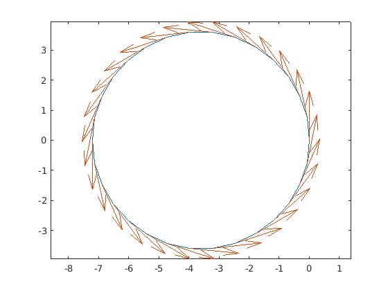
A trajectory controller requires a path to follow with characteristics at each point in the path of (i) position in (x,y), and (ii) the desired orientation along the path at that point. In the above plot, you can see the desired orientation at each point, indicated as the vector arrows.
Controller design
The controller as implemented is taken from a controller developed by Hoffmann, and described in [1] below. The controller requires three basic inputs:
- The nearest point on the trajectory
- The desired heading at that point
- The desired velocity
The controller combines with these three state values, the following values obtained through access to the simulation:
- The cross-track error (obtained from 1)
- The heading error (obtained from (1) and (2))
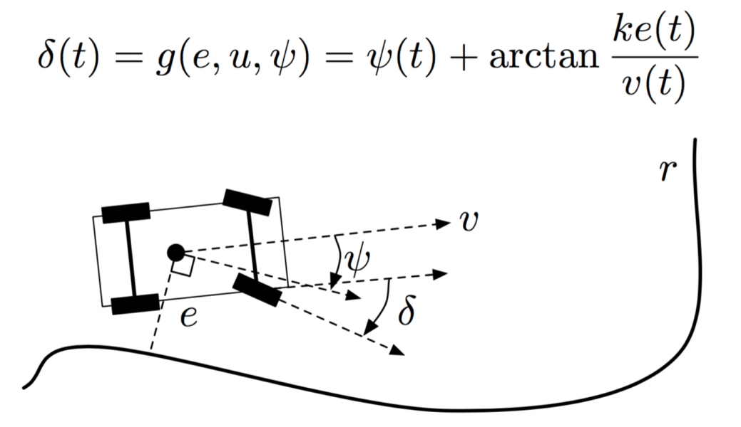
Using these values, it solves for the desired steering angle as described in [1]. A diagram of this behavior is shown below.
Implementation in Simulink
The simulink model is developed hierarchically.
Model overview

In the overview we see the state data obtained from odometry information. We provide a reference velocity of 3 m/s, and the path is pre-programmed in the "Select desired path". We also create here the output message (geometry/Twist) and publish it to the topic of /catvehicle/cmd_vel. Note that the other published data of /catvehicle/waypoint are not in use.
Hoffmann Controller Implementation

You see here how the (x,y,heading) are obtained from odometry data, and path is obtained as the desired setting. We see how to obtain the various errors inside of "calculate e": note that we actually only need e and its sign, the other values are if you want to plot the nearest point as part of debug information.
% calculate e matlab function

		function [e,phipath,xpathOut,ypathOut] = fcn(x,y,pathV)

		%#codegen

		path=reshape(pathV,[],3);

		x1 = path(1,1);

		y1 = path(1,2);

		phi1=path(1,3);

		etmp = inf;

		e = inf;

		index=1;

		% find the nearest x,y

		for i=1:length(path)

		   etmp = sqrt((x-path(i,1))^2+(y-path(i,2))^2);

		   if( etmp < e )

		       e = etmp;

		       index=i;

		   end

		end xpathOut=path(index,1);

		ypathOut=path(index,2);

		phipath=path(index,3);


		ex1 = (path(index,1)-x);

		ey1 = (path(index,2)-y);

		ex2 = cos(phipath);

		ey2 = sin(phipath);

		sinnnn = ex1*ey2-ey1*ex2;

		e = sign(sinnnn)*e;
The other function of interest implements the Hoffmann controller:
% calculate delta
function delta = fcn(k,e,v,phi)
%#codegen
if( abs(v) < eps )
v = eps;
end
% if phi is greater than pi (or less than -pi), then
% we normalize to between [-pi,pi]
if( phi < -pi )
phi = phi+2*pi;
elseif( phi > pi )
phi = phi-2*pi;
end
delta = phi + atan2(k*e,v);
Safety control
The switch that guards vOut changes the velocity to 0 if the vehicle's odometry measures it to be more than 4m away from the path**. This is intended to assist in debugging by preventing the vehicle from driving in such a way as to indicate controller error when in fact it is just far away from the trajectory.
Starting the controller
Once you have started the simulation and visualization tool, you need only start up the controller:
You will now see the car driving in a circle---it will do this as long as you let it. If you want to see where it has driven, and its current odometry information, subscribe in the Displays panel in rviz to add (by topic):
- /catvehicle/odom
- /catvehicle/path
References
The provided implementation is developed using the presentation in [1]. The Simulink implementation is developed using the Robotics System Toolbox.
[1] Sebastian Thrun, et al. 2006. "Stanley: The robot that won the DARPA Grand Challenge" Research Articles. J. Robot. Syst. 23, 9 (September 2006), 661-692. DOI=http://dx.doi.org/10.1002/rob.v23:9
** There is actually a flaw in the design here, can you spot it?
azcar_sim (deprecated)
The below is a deprecated version of the APIs and will be removed.
Overview
In this tutorial we will demonstrate how to follow a trajectory using a controller. In this case, the controller was developed in MATLAB/Simulink, and the generated code is provided as part of the release.
Starting up the simulation
For this launch, I will use the skidpan so as to ensure that we do not encounter any obstacles through the trajectory we will be trying to follow.
$ roslaunch azcar_sim azcar_skidpan.launch
For this simulation, I recommend using rviz so we can vizualize the vehicle's odometry and path.
$ rosrun rviz rviz
And load your .rviz file which will help you visualize the sensor data.
Understanding the trajectory
The trajectory we follow is a circle of radius, which starts at position [0 0] (this is the initial position of the vehicle in most simulations). If you have a copy of MATLAB, you can run the provided file in src/azcar_sim/simulink/circularPathPrototype.m and see the plot of the desired trajectory. The plot is produced here:
A trajectory controller requires a path to follow with characteristics at each point in the path of (i) position in (x,y), and (ii) the desired orientation along the path at that point. In the above plot, you can see the desired orientation at each point, indicated as the vector arrows.
Controller design
The controller as implemented is taken from a controller developed by Hoffmann, and described in [1] below. The controller requires three basic inputs:
The nearest point on the trajectory
The desired heading at that point
The desired velocity
The controller combines with these three state values, the following values obtained through access to the simulation:
The cross-track error (obtained from 1)
The heading error (obtained from (1) and (2))
Using these values, it solves for the desired steering angle as described in [1]. A diagram of this behavior is shown below.
[Visual depiction of Hoffmann steering controller logic.]
Implementation in Simulink
The simulink model is developed hierarchically.
Model overview
In the overview we see the state data obtained from odometry information. We provide a reference velocity of 3 m/s, and the path is pre-programmed in the "Select desired path". We also create here the output messag (geometry/Twist) and publish it to the topic of /azcar_sim/cmd_vel. Note that the other published data of /azcar_sim/waypoint are not in use.
Hoffmann Controller Implementation
You see here how the (x,y,heading) are obtained from odometry data, and path is obtained as the desired setting. We see how to obtain the various errors inside of "calculate e": note that we actually only need e and its sign, the other values are if you want to plot the nearest point as part of debug information.
% calculate e matlab function function [e,phipath,xpathOut,ypathOut] = fcn(x,y,pathV) %#codegen path=reshape(pathV,[],3); x1 = path(1,1); y1 = path(1,2); phi1=path(1,3); etmp = inf; e = inf; index=1; % find the nearest x,y for i=1:length(path) etmp = sqrt((x-path(i,1))^2+(y-path(i,2))^2); if( etmp < e ) e = etmp; index=i; end end xpathOut=path(index,1); ypathOut=path(index,2); phipath=path(index,3); ex1 = (path(index,1)-x); ey1 = (path(index,2)-y); ex2 = cos(phipath); ey2 = sin(phipath); sinnnn = ex1*ey2-ey1*ex2; e = sign(sinnnn)*e;
The other function of interest implements the Hoffmann controller:
% calculate delta function delta = fcn(k,e,v,phi) %#codegen if( abs(v) < eps ) v = eps; end % if phi is greater than pi (or less than -pi), then % we normalize to between [-pi,pi] if( phi < -pi ) phi = phi+2*pi; elseif( phi > pi ) phi = phi-2*pi; end delta = phi + atan2(k*e,v);
Safety control
The switch that guards vOut changes the velocity to 0 if the vehicle's odometry measure it to be more than 4m away from the path**. This is intended to assist in debugging by preventing the vehicle from driving in such a way as to indicate controller error when in fact it is just far away from the trajectory.
Starting the controller
Once you have started the simulation and visualization tool, you need only start up the controller:
rosrun hoffmannfollower hoffmannfollower_node
You will now see the car driving in a circle---it will do this as long as you let it. If you want to see where it has driven, and its current odometry information, subscribe in the Displays panel in rviz to add (by topic):
/azcar_sim/odom
/azcar_sim/path
References
The provided implementation is developed using the presentation in [1]. The Simulink implementation is developed using the Robotics System Toolbox.
[1] Sebastian Thrun, Mike Montemerlo, Hendrik Dahlkamp, David Stavens, Andrei Aron, James Diebel, Philip Fong, John Gale, Morgan Halpenny, Gabriel Hoffmann, Kenny Lau, Celia Oakley, Mark Palatucci, Vaughan Pratt, Pascal Stang, Sven Strohband, Cedric Dupont, Lars-Erik Jendrossek, Christian Koelen, Charles Markey, Carlo Rummel, Joe van Niekerk, Eric Jensen, Philippe Alessandrini, Gary Bradski, Bob Davies, Scott Ettinger, Adrian Kaehler, Ara Nefian, and Pamela Mahoney. 2006. "Stanley: The robot that won the DARPA Grand Challenge" Research Articles. J. Robot. Syst. 23, 9 (September 2006), 661-692. DOI=http://dx.doi.org/10.1002/rob.v23:9
** There is actuall a flaw in the design here, can you spot it?